DASC 240 intro

Professor McNamara

Amelia McNamara (she/her)

prefer to be called “Dr. McNamara” or “Professor McNamara”(pronounced “MacNamera”)

amelia.mcnamara@stthomas.edu

OSS 407

Office hours:

• Mondays 11 am- noon (Zoom)
• Fridays 1-2 pm (Zoom)
• Or by appointment (Zoom)

About me

Bachelor’s degree in English and mathematics, PhD in statistics from UCLA.

Outside of work I like reading fiction, weightlifting, working on my house (and old car!), and darning (a method of repairing knitted garments).

I live in Minneapolis with my husband and dog (Bentley).

Introductions

I’d love for everyone to introduce themselves

• Name/pronouns
• Major and class year
• An interest or hobby

Why am I still masking?

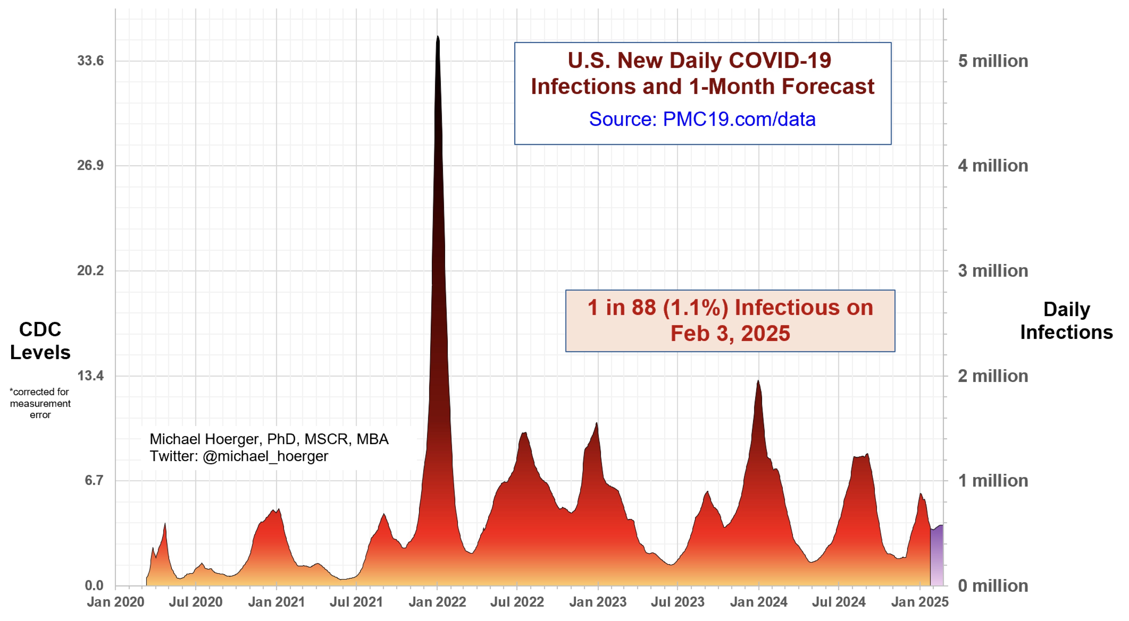
A “mass disabling event”

“Some researchers have estimated that 10% to 35% of people who have had COVID-19 went on to have long COVID.”

“Studies estimating its prevalence in pediatric populations are limited and conflicting, estimating up to 25% of children infected with the SARS-CoV-2 virus could go on to develop long COVID. A study published in 2024 estimated that up to 5.8 million young people have long COVID.”

via https://www.mayoclinic.org/diseases-conditions/coronavirus/in-depth/coronavirus-long-term-effects/art-20490351 and https://www.salon.com/2024/08/26/long-is-a-public-health-for-kids-experts-say/

What can we do?

What’s wrong with generative AI?

• It’s consumptive
• It’s not transformative
• It doesn’t “know” anything”
• It damages the environment

Okay, back to this class

What are models?

• A simplification of the world

  • Physics joke– imagine a spherical cow

• Mathematical and statistical models

  • Math models: create a model of the world, use the model to generate data, look at the data and see if it looks like the world

  • Statistical models: collect data from the world, use the data to fit a model, and look to see how well the model fits the data

Why do we make models?

• understand/describe the world

• predict things

  • within the range of the data

  • in the future

Data and variables review

Model inputs and outputs

Statistical language

Thinking about data (links on Canvas)

• How many explanatory variables? Are they categorical or quantitative?
• What is the response variable? Is it categorical or quantitative?
• What is the model being used for? Prediction? Description?

Software in this course

We’ll be using R and RStudio throughout the course to learn statistical concepts and analyze real data to come to informed conclusions.

What is R?

R is a programming language specifically designed for statistical analysis. R is open-source, and is developed by a team of statisticians and programmers in both academia and industry. It is updated frequently and has become the de facto industry standard. In the data science realm, alternatives to R include Python with the pandas library, and Julia. In the statistics realm, alternatives include SAS, Stata, and SPSS.

What is RStudio?

RStudio is an Integrated Development Environment (IDE) for R. RStudio is also open-source software, and depends upon a valid R installation to function. RStudio as available as both a both Desktop and Cloud application. Before RStudio, people used R through the command line directly, or through graphical user interfaces like Rcmdr, but RStudio is so vastly superior that these alternatives have few users left. RStudio employees are important drivers of R innovation, and currently maintain packages like ggplot2, dplyr and tidyverse, among others.

What is Quarto?

Quarto is format for composing relatively simple documents that combine code and text. Quarto relies on a version of markdown (a general-purpose authoring format), and provides functionality for processing code and including the output. We’ll be using Quarto with R code chunks, but it also works with Python, Julia, and other programming languages.

The RStudio interface

The panel in the upper right contains your environment as well as a history of the commands that you’ve previously entered. Any plots that you generate will show up in the panel in the lower right corner.

The panel on the left is where the action happens. It’s called the console. Every time you launch RStudio, it will have the same text at the top of the console telling you the version of R that you’re running. Below that information is the prompt. As its name suggests, this prompt is really a request, a request for a command. Initially, interacting with R is all about typing commands and interpreting the output. These commands and their syntax have evolved over decades (literally) and now provide what many users feel is a fairly natural way to access data and organize, describe, and invoke statistical computations.

Getting ready: RStudio project

It’s important to have a good file organization structure for this class. RStudio has a feature called “Projects” that are basically special folders on your computer RStudio knows a lot about. Let’s make a project for this course. In RStudio, go to

File ->

New Project ->

New Directory¹ ->

New Project ->

Pick a directory name (maybe DASC240, all one word) ->

Pick where the directory will live (I highly suggest OneDrive) ->

Create Project

RStudio should restart and you should then see the name of your project in the upper right corner of RStudio.

1. Unless you already have a folder created for this class

Getting ready: RStudio settings

The default settings in RStudio are mostly pretty good! But, there are a couple I like to change. Let’s do that. Go to:

Tools ->

Global Options

On the General page, change “Save workspace to .RData on exit” to “Never” On the RMarkdown page, uncheck “Show output inline in RMarkdown documents” If you prefer a different color scheme, check out the Appearance page

When you’re done setting things up, hit Okay.

Trying out R

To get started, enter all commands at the R prompt (i.e. right after > on the console); you can either type them in manually or copy and paste them from this document.

At its simplest, R is just a big calculator. So, it can do arithmetic and apply functions.

2+2
100/10
log(100)
sqrt(100)

R packages

R has a number of additional packages that help you perform specific tasks. For example, dplyr is an R package designed to simplify the process of data wrangling, and ggplot2 is for data visualization based on the Grammar of Graphics (a famous book).

In order to use a packages, they must be installed (you only have to do this once) and loaded (you have to do this every time you start an R session).

Installing packages

To be able to do more advanced stuff, you need additional packages. I have a list of them on Canvas, which you can install by copy-pasting into the Console and hitting enter.

install.packages(c("agricolae","babynames", "car", "devtools", "forecast", 
                    "fueleconomy", "GGally","Hmisc", "infer", "ISLR", 
                    "janitor", "leaps", "lmtest", "Lock5Data","manipulate",
                    "mosaic", "nnet", "nycflights13", "skimr", "Stat2Data", 
                    "tidymodels", "tidyverse", "usethis"))

A bunch of red text will scroll by, which mean it’s working! Installing all the packages may take a few minutes; you’ll know when the packages have finished installing when you see the R prompt (>) return in your console.

Loading packages

The additional packages we installed will help you perform specific tasks. We’ve already installed them, which only needs to be done once. In order to use a package we have to load it. This needs to happen every time you start an R session. To load a package, you use the library() command,

library(tidyverse)

── Attaching core tidyverse packages ──────────────────────── tidyverse 2.0.0 ──
✔ dplyr     1.1.4     ✔ readr     2.1.5
✔ forcats   1.0.0     ✔ stringr   1.5.1
✔ ggplot2   3.5.1     ✔ tibble    3.2.1
✔ lubridate 1.9.3     ✔ tidyr     1.3.1
✔ purrr     1.0.2     
── Conflicts ────────────────────────────────────────── tidyverse_conflicts() ──
✖ dplyr::filter() masks stats::filter()
✖ dplyr::lag()    masks stats::lag()
ℹ Use the conflicted package (<http://conflicted.r-lib.org/>) to force all conflicts to become errors

You might get a “message” when you load a package, but otherwise not much happens. But, then it’s ready for us to use! The tidyverse package loads many useful packages for data analysis and visualization.

Loading data

Some packages come with data built into them, which we can load into our Environment using the data() function. Let’s try loading in the diamonds data.

data(diamonds)

Some datasets immediately get loaded into the Environment, but many datasets (especially big ones) are ‘lazy loaded,’ which means you need to do something with them in order for R to load them in. One thing to do is to click on the name of the dataset.

Observations and variables

• What are the observational units in the diamonds data? How many are there?
• What are the variables?
• Are there any categorical variables? Quantitative variables? Can you make more fine-grained distinctions for the variable types?

If you have questions about a built-in dataset, you can use the ? operator to learn more about it.

?diamonds